Way back in Week 1, we learned that an algorithm is nothing more than a set of instructions given to the computer.
This week will broaden our understanding of algorithms as we traverse arrays, searching and sorting their elements.
Recall that we can qualify code by its correctness, design, and style. Week 3 hones in on design, or the efficiency of a program, which is measured by how fast it runs.
As always, this guide will be split into two parts: my personal notes and thoughts on the course content, along with my experience with the week’s problem set.
Lecture Notes
To recap, arrays are blocks of memory stored side-by-side, sort of like a locker.
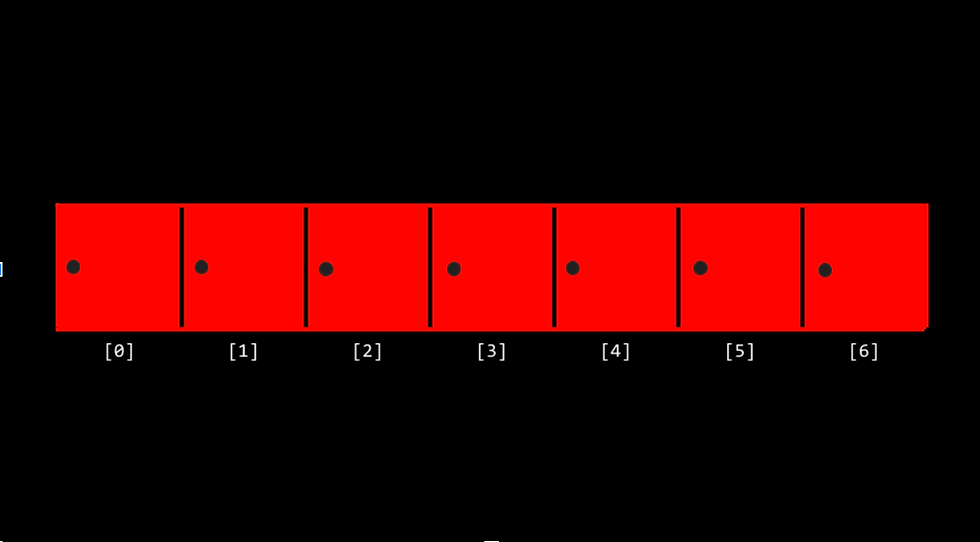
Behind each of these seven doors is a distinct ‘value’, very much akin to how arrays store data within each adjacent block of memory.
With this in mind, let’s break down Week 3.
Search Algorithms
So what if we wanted to find out if a certain number, say the number 35, is stored behind one of those doors?
Well, we could implement a simple search algorithm. Before we start writing in C, however, it’s always good practice to start off with pseudocode.
We might tackle this problem by traversing the array – opening each door one-by-one – and then checking whether 35 appears behind one of those doors.
If so, the program would return true, and if not, false.
For each door from left to right
If 35 is behind door
Return true
Return false
Taking this pseudocode one step further, from human-readable instructions to a close approximation of the final code, we might end up with the following.
For i from 0 to n-1
If 35 is behind doors[i]
Return true
Return false
Even the phone book scenario we explored in Week 0 is an example of a search algorithm, more specifically, a binary search algorithm.
Binary search algorithms, assuming that all values within an array have been arranged in increasing order, follow a ‘divide-and-conquer’ approach – breaking a larger problem into smaller ones until your solution remains.
With this in mind, let’s circle back to our original problem using binary search.
If no doors
Return false
If 35 is behind doors[middle]
Return true
Else if 35 < doors[middle]
Search doors[0] through doors[middle-1]
Else if 35 > doors[middle]
Search doors[middle+1] through doors[n-1]
Here, we begin by immediately checking whether the array exists, and returning false if not.
If the array does exist, however, we proceed by determining if 35 appears in the middle index of the array.
If not, knowing that the numbers are arranged in ascending order, we next check if 35 is less than the middle value or greater, and search the respective doors (the left half, if 35 appears to the left of the middle, and the right half, if 35 appears to the right).
Notice how we can almost express this pseudocode formally in the C language, perhaps aside from the recursive function ‘search’, which Week 3 will touch upon later.
Time Complexity with Big O Notation
Let’s revisit this time complexity graph from Week 0’s phonebook algorithm.
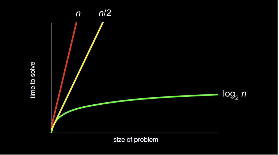
You might have noticed that the yellow and red lines are labeled with the same ‘O(n)’ when their slopes are markedly different.
Big O notation describes the upper bound of a program’s runtime, meaning that if you zoomed out really, really far, the yellow and red lines would seem to overlap each other.
Although in reality the yellow line has a time complexity of n/2, the coefficient is negligible as we really only focus on the main factor influencing the time to solve an algorithm.
Accordingly, log₂n is written in Big O notation as O(logn), as the change of base formula for logarithms leaves us with a constant of 1/log2, which can be disregarded.
Common runtimes seen across algorithms include:
O(n2)
O(nlogn)
O(n)
O(logn)
O(1)
Try to envision the rough shape of each graph in relation to one another.
As the size of the problem increases, graphs that increase at relatively faster rates than others are regarded as bad running times.
Of the above examples, constant runtimes, like O(1), are the fastest, and exponential runtimes, like O(n2) are generally the worst.
Note that Big O notation is a measure of the slowest possible runtime a program could have.
But programmers don’t always see the glass as half-empty!
To indicate the lower bound, or best case scenario, of an algorithm, the 𝛺 symbol is used instead of O.
Say in a linear search algorithm, assuming a sorted list of integers, the number we are looking for appears first, the program would terminate at one step; thus, in Big Omega notation, the runtime for this program could be written as 𝛺(1).
Finally, if both 𝛺 and O are the same – that is to say, if both the upper and lower bound of an algorithm are the same – we can express the runtime in Big Theta notation using the 𝛳 symbol.
Linear Search Algorithms
Now that we have a general idea of how search algorithms work, let’s try to implement one of our own in the CS50 codespace!
Let’s suppose we were provided an array of integers with the goal of searching for a user-inputted number. A potential solution could look something like this:
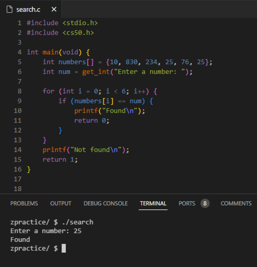
Here, an array of integers numbers is initialized with 6 values, and the variable num requests a number from the user.
In the for loop is where we can find an implementation of a linear search algorithm – the loop traverses all elements within the array, from indexes zero to five, checking whether each list item is, indeed, our num.
Notice how we can calculate the time complexity of this algorithm by determining how many conditions would need to be checked in the best and worst cases.
For instance, if (optimally) num appeared at the array’s zeroth index, the program would return 0 and terminate at the loop’s first cycle – this lower bound can be expressed as
𝛺(1).
Conversely, if num was the last element in the list or even did not appear in the list at all, the program would terminate after running n times (n being the length of the list) – this upper bound can be expressed as O(n).
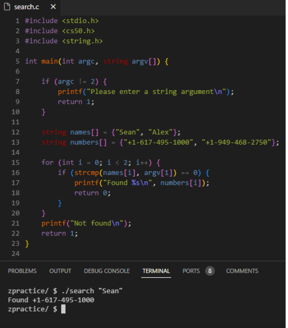
Implementing linear search is, for the most part, no different for other data types. Let’s replicate this process using a string array.

To make this program slightly more interesting and incorporate concepts from Week 1, I’ve used command line arguments as a substitute for CS50’s ‘get_string()’ function.
Oddly enough, when comparing strings, the == operator will not suffice – the compiler interprets this as comparing the memory location of the string with the list element, as opposed to the value.
Luckily, including the string.h library and using strcmp() solves this issue.
So what would happen if we combined both strings and numbers in an (admittedly short) phonebook?
While this code technically works, it’s good practice to consider factors other than correctness – namely, design.
This program assumes that any given index within names and numbers correspond to one another. But what if, for example, someone doesn’t have a number?
Or perhaps a name or number gets misaligned?
What if we could connect both arrays to make names and numbers operate as just one array?
Custom Data Types
To our convenience, C allows us to define our own data structures using the following syntax:
typedef struct
{
string name;
string number;
}
person;
To call a struct a custom data type would be a bit of a misnomer – in reality, all we’re really doing is mashing multiple existing data types into just one.
In the example above, the struct is initialized by the keywords ‘typedef struct’.
Within the following curly braces is where we would define the properties of our data type – here, the struct is given two string variables, name and number.
Finally, the struct is closed off with the name of the data type. As per usual, it’s the convention to name your type something descriptive and accurate.
In this case, we’ve defined person as anything with a name and a number.
Let’s return to our phone book problem.
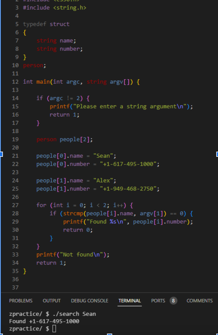
Some modifications made to our original, poorly-designed program:
Our struct person was declared outside of the main() function
A new array people was created of type person and of size two
In order to access each individual data type within person, we first had to index into each individual array element, and then use dot notation to access the name or number component (people[0].name)
Regardless of whether or not name or number was fitted with a value, the program would still work!
Sorting Algorithms
Like most things computer-related, the algorithmic process of sorting values is vastly different than the intuitive approach humans would take.
Professor Malan invites eight volunteers to the stage to sort themselves, which they were able to do with ease.

Unfortunately, code runs line-by-line, meaning only one condition is checked at a time (as opposed to different numbers comparing themselves all at once like in the demonstration).
Sorting – that is, inputting an unsorted list of values and outputting a sorted one – can be used to improve design (by optimizing runtime) when searching a list for values.
For instance, binary search can only be used on a sorted list, as it relies on where the desired value lies in relation to other values in the list.
One such sorting algorithm is selection sort.
For i from 0 to n–1
Find smallest number between numbers[i] and numbers[n-1]
Swap smallest number with numbers[i]
We can use this algorithm to sort the list of numbers shown on the projector of the image above.
5 2 7 4 1 6 3 0
0 | 2 7 4 1 6 3 5
0 1 | 7 4 2 6 3 5
0 1 2 | 4 7 6 3 5
This process of traversing the array, finding the smallest number within a decreasing range, and swapping the number of position i with that smallest value repeats until the list is fully sorted…
0 1 2 3 4 5 6 | 7
Mathematically, we can calculate the upper and lower bounds of the selection sort algorithm.
The loop that first appears iterates from 0 to n-1 – that is,
n times.
Within the loop, a simpler algorithm for finding the smallest number iterates over the loop (n-1) + (n-2) + (n-3) + … + 1 times over the course of the outer for loop – in other words, (n-1)!
Expressing this factorial as a summation and simplifying, we get n2/2 - n/2.
Finally, factoring in the swap algorithm, we can assume that it will yield kn steps, where k is some constant.
Summing up the two equations, we get n2/2 - n/2 + kn, and because n2 is the most influential factor in determining the runtime of this algorithm, we can say that selection sort is of the order O(n2).
Note that in this algorithm, there is no conditional statement that, if true, breaks out of the loop like in our linear search implementation.
Thus, even if all the values in the list were pre-sorted, the lower bound would also be 𝛺(n2). And because the upper and lower bounds are equal, we can express this algorithm’s runtime in Big Theta notation 𝛳(n2).
Another sorting algorithm is called bubble sort, in which two elements within a ‘bubble’ are swapped based on their value.
Terminate is set to true
Repeat n-1 times
For i from 0 to n–2
If numbers[i] and numbers[i+1] out of order
Swap them
Terminate is set to false
If terminate is set to true
Return 0
Else
Terminate is set to false
A more palatable version of this pseudocode can be found below, however it loses the ability to break out of the loop early, compromising on the algorithm’s runtime.
Repeat n-1 times
For i from 0 to n–2
If numbers[i] and numbers[i+1] out of order
Swap them
Using the same unsorted list:
5 2 7 4 1 6 3 0
2 5 7 4 1 6 3 0
2 5 7 4 1 6 3 0
2 5 4 7 1 6 3 0
2 5 4 1 7 6 3 0
2 5 4 1 6 7 3 0
2 5 4 1 6 3 7 0
2 5 4 1 6 3 0 | 7
Notice how after one iteration of the for loop, we’ve successfully brought the greatest element to the end of our array, thus, one step closer to sorting it. After this loop has run n times, we will be left with a sorted list of numbers…
0 1 | 2 3 4 5 6 7
Again, let’s express this algorithm using Big O and Big Omega notation.
The blanketing for loop repeats from zero to n-2 a total of n-1 times.
The inner loop repeats from zero to n-2, yielding, again, n-1 total runs.
In the worst case scenario, when the size of the problem is at its largest, we know that every adjacent element will be out of order. Thus, the if-statement will evaluate to true and both values will swap for every iteration – for simplicity’s sake, we can assume that this will take k(n-1)2 steps (as swapping two values will result in some constant k number of steps).
Similarly, in the best case, the array will come fully sorted. Therefore, upon checking whether the adjacent elements are out of order and evaluating to false each time within the for loop, the boolean variable terminate will remain true.
In the subsequent line, because terminate is true, the algorithm will return zero, the program only having run k(n-1) times.
Extracting the most influential term from both the upper and lower bounds, we can express bubble sort’s time complexity as O(n2) and 𝛺(n).
Recursion and Merge Sort
Recursion is when a function or method calls itself. Sounds a little paradoxical, right? How can a function keep calling itself without getting stuck in an infinite loop…?
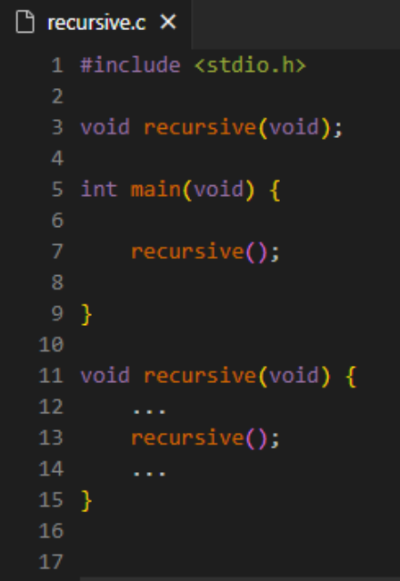
This (obviously incomplete) function ‘recursive()’ is something similar to what you might encounter when dealing with recursive functions in C. So how is this type of function any practical?
It turns out we’ve, rather unknowingly, already used recursive functions in our pseudocode implementation of binary search.
If no doors
Return false
If number behind middle door
Return true
Else if number < middle door
Search left half
Else if number > middle door
Search right half
The ‘search()’ function is called over and over, within itself, with new parameters, eventually returning false or true, thus terminating the loop.
Consider Week 1’s pyramid structure algorithm.
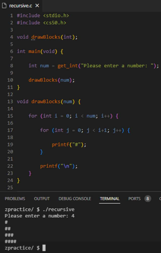
While, of course, this program works, let’s try to make it recursive.
Within ‘drawBlocks()’, the function continues to call itself with one height less each time, resulting in the smallest height being called first, all the way up until there are num blocks in the last row.
To envision this more clearly, imagine that we’ve replaced the recursive ‘drawBlocks(num - 1)’ call with the contents of the function up until the base case, num - 1 > 0, evaluates to false.
A base case condition ensures that the function doesn’t get stuck in an infinite loop, and that height is always a positive integer.
So really, when the function is called in main() with a height of four, the code that is being run is, quite simply:
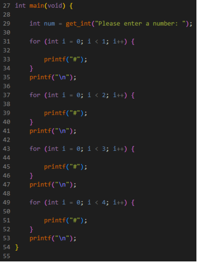
With recursion in mind, we can now go about implementing one of the most efficient sorting algorithms there is – merge sort.
The strategy with merge sort is to sort one half of the array and the other, and then merge them together until just one number remains, after which we cannot split the array into halves.
If only one number
Quit
Else
Sort left half of number
Sort right half of number
Merge sorted halves
Let’s test this out on a list of numbers.
7 2 5 4
Because this list contains more than one value, our program will go ahead and split the numbers down the middle.
7 2 | 5 4
On the left and right sides, the program will continue splitting the increasingly smaller arrays in half, until splitting the array will result in one number, by which time it will sort the two numbers on the left, and the two numbers on the right.
2 7 | 4 5
With both halves sorted, the algorithm will merge both sides, comparing element zero in the left array with element zero in the right array, and putting the smaller of the two first in the final list, and then the second smallest. This process will repeat until the array is fully sorted!
2 4 5 7
Because merge sort must visit every place in the list in the best and worst cases, its time complexity can be written as
𝛳(nlogn), making it highly efficient in sorting large sets of data.
Problem Set 3: Plurality
This week’s problem set has us simulate a plurality vote election, in which each user casts a ballot, so to speak, of a valid candidate, and then the program returns the candidate, or candidates, with the greatest number of votes.
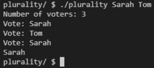
Sarah and Tom are the candidates here, fed to the program as command-line arguments. Because Sarah received more votes than Tom, her name was printed at the end.
Some corner cases include casting a vote for non-existent candidates and multiple candidates holding the most votes.
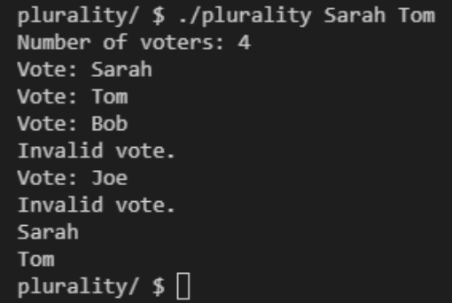
Note how both Sarah and Tom were printed at the end, as they both received one vote, and that votes that were deemed ‘invalid’ were not counted.
With the technicalities out of the way, let’s enumerate each section of Plurality, beginning with declarations.
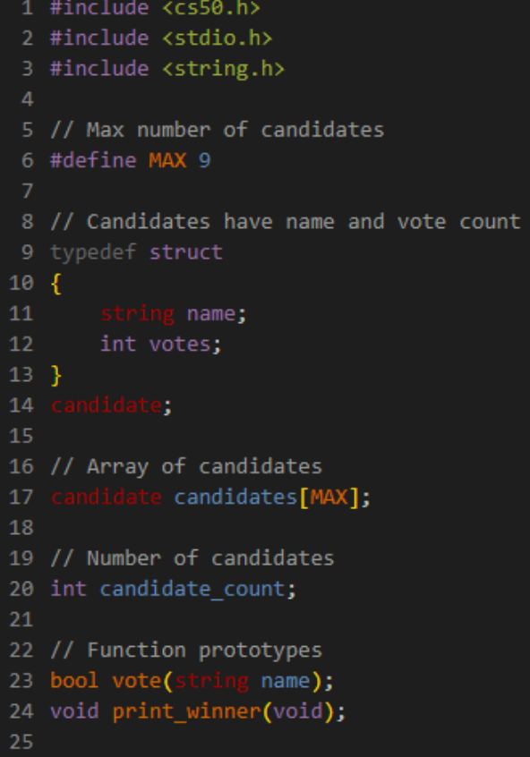
After including all of the necessary libraries within our file, we stumble upon this cryptic ‘#define’ syntax followed by a capitalized variable, MAX, and an int, ‘9’.
All this line is doing is assigning the value ‘9’ to a constant and unchangeable variable, MAX. Typically in C, the convention is to capitalize variables which remain constant.
Within the struct provided, we know that the candidate data type is made up of a string and an int.
Finally, line 17 initializes an array of candidates of size nine (the value stored within MAX) and a few function prototypes are declared so as to be used later on.
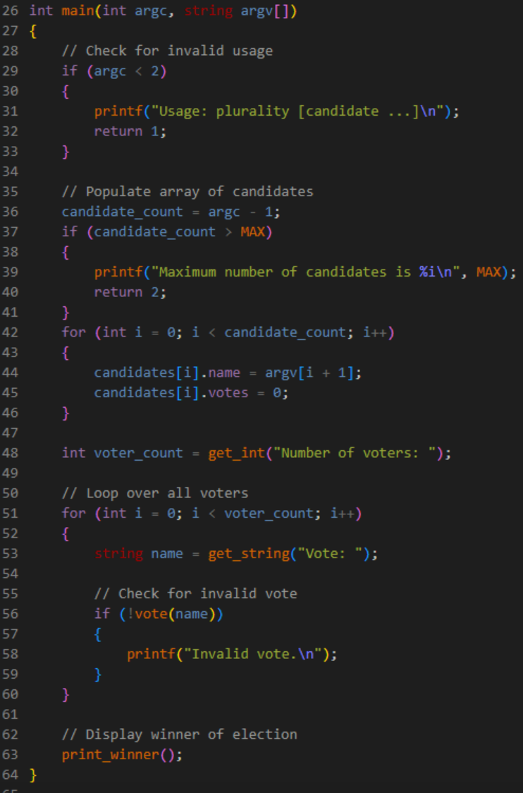
Within the main() function, the program begins by checking for the appropriate amount of command-line arguments, exiting the program if no candidate names are entered.
Recall that argc stores the value of all terminal arguments, including ‘./plurality’, meaning that the total number of candidates entered by the user can be determined by argc - 1 (not exceeding MAX, or nine).
In order to ‘populate’ the empty candidates array, we can loop over argv, an array that stores all command-line argument values.
Every time this array is looped over, that is to say argc-1 times, we access the ith index of candidates, storing the value of each candidate as name using dot notation.
Note how we must add 1 to the index of argv to avoid accessing ‘./plurality’.
Finally, the number of voters is retrieved from the user, and for each voter, if name does not match any of the candidates, then that vote is considered invalid.
Oddly enough, line 56 calls the vote() function, expecting a boolean – true or false – return. Let’s implement vote().
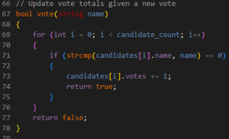
The purpose of vote is to add a vote to a candidate if their name appears as an option.
The for loop traverses the candidates array candidate_count, or argc-1, times, using the strcmp() function to compare the value of the string parameter name with every candidate in the candidates array.
If such a candidate name was found, vote() would return true, and if upon traversing the array, name was not one of the candidate options, vote() would return false.
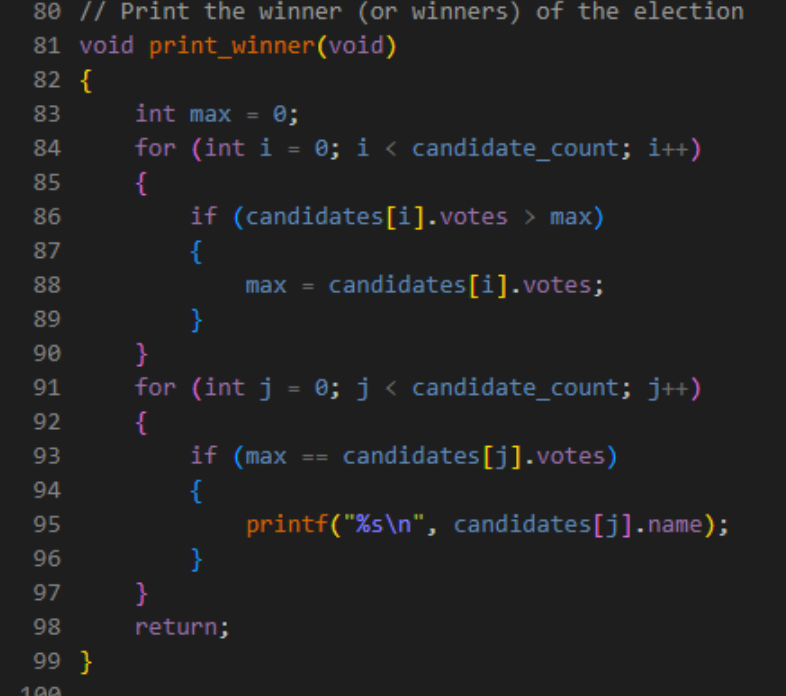
After tallying up all the votes, the only thing left to do is to print the election winner.
print_winner() finds the largest value of votes among all of the candidates, and then prints the names of the candidates with the corresponding votes.
Each time a greater value of votes is found, the variable max is updated to store the greatest number of votes in the array.
The subsequent loop checks for which candidate names the maximum votes corresponds with, and then prints each respective name.
While using two loops may seem redundant and unnecessary here, they are, indeed, needed – if there were multiple candidates with the same maximum number of votes, every candidate in the array with that vote must be printed.
Final Thoughts
In some form or another, algorithms will play a part in your life, whether you choose to pursue programming or not.
As for the next couple of weeks, as CS50x delves deeper into memory and data structures, don’t expect the coursework and coding process to be as simple as
O(1)!
That’s it for Week 3.
Note: this article has images and code belonging to CS50. You are free to you remix, transform, or build upon materials obtained from this article. For further information, please check CS50x’s license.
Comentarios